The data sources available in the dropdowns and the way A4 is calculated depend on the project’s country and calculation type. See Methodology & Compliance for the rules.
Page layout
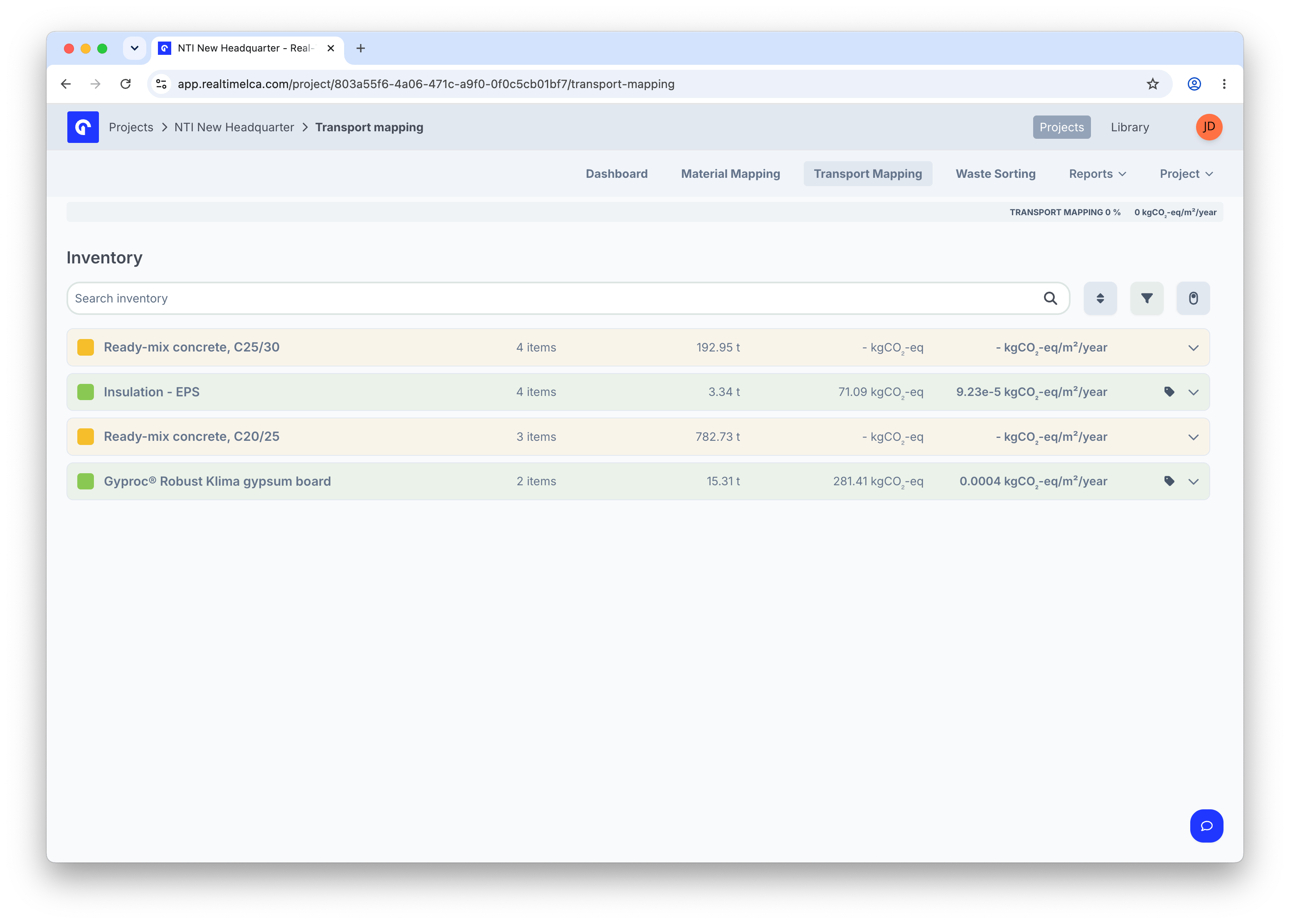
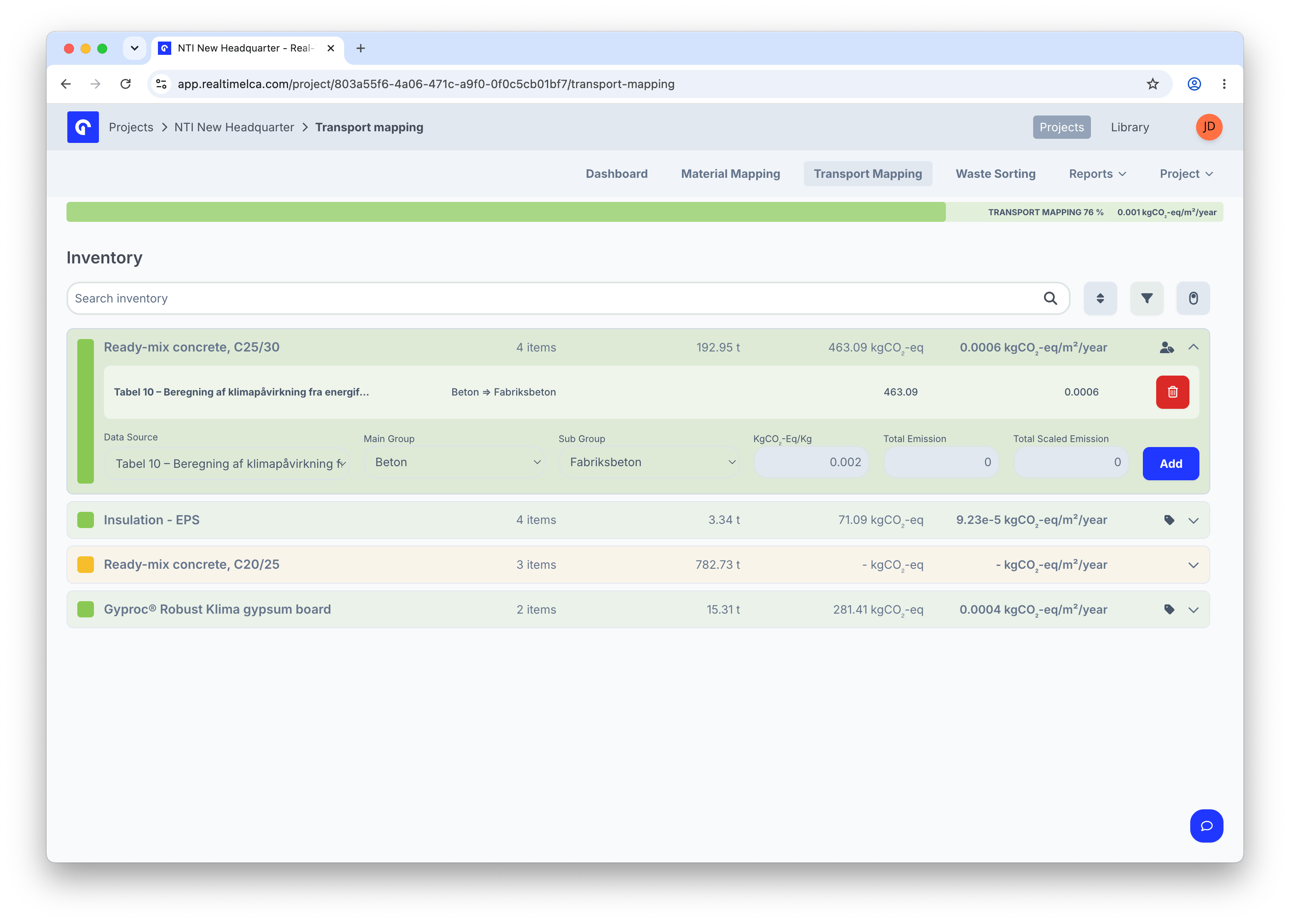
Transport Mapping uses a single panel — there is no Library to drag from. Each row in the Inventory is one of the materials already mapped in Material Mapping, with a quantity and a colour that tells you the row’s state at a glance. The header strip shows two live numbers:- TRANSPORT MAPPING % — share of inventory rows that have a transport assignment.
- kgCO₂-eq/m²/year — current A4 intensity based on what is already mapped.
Row states
| Colour | Meaning |
|---|---|
| Green | A4 emissions are covered — either by an assigned transport type or because the EPD’s data already includes A4 (see Material-derived data source). |
| Yellow | The row is unmapped. A4 will be zero until you assign a transport type. |
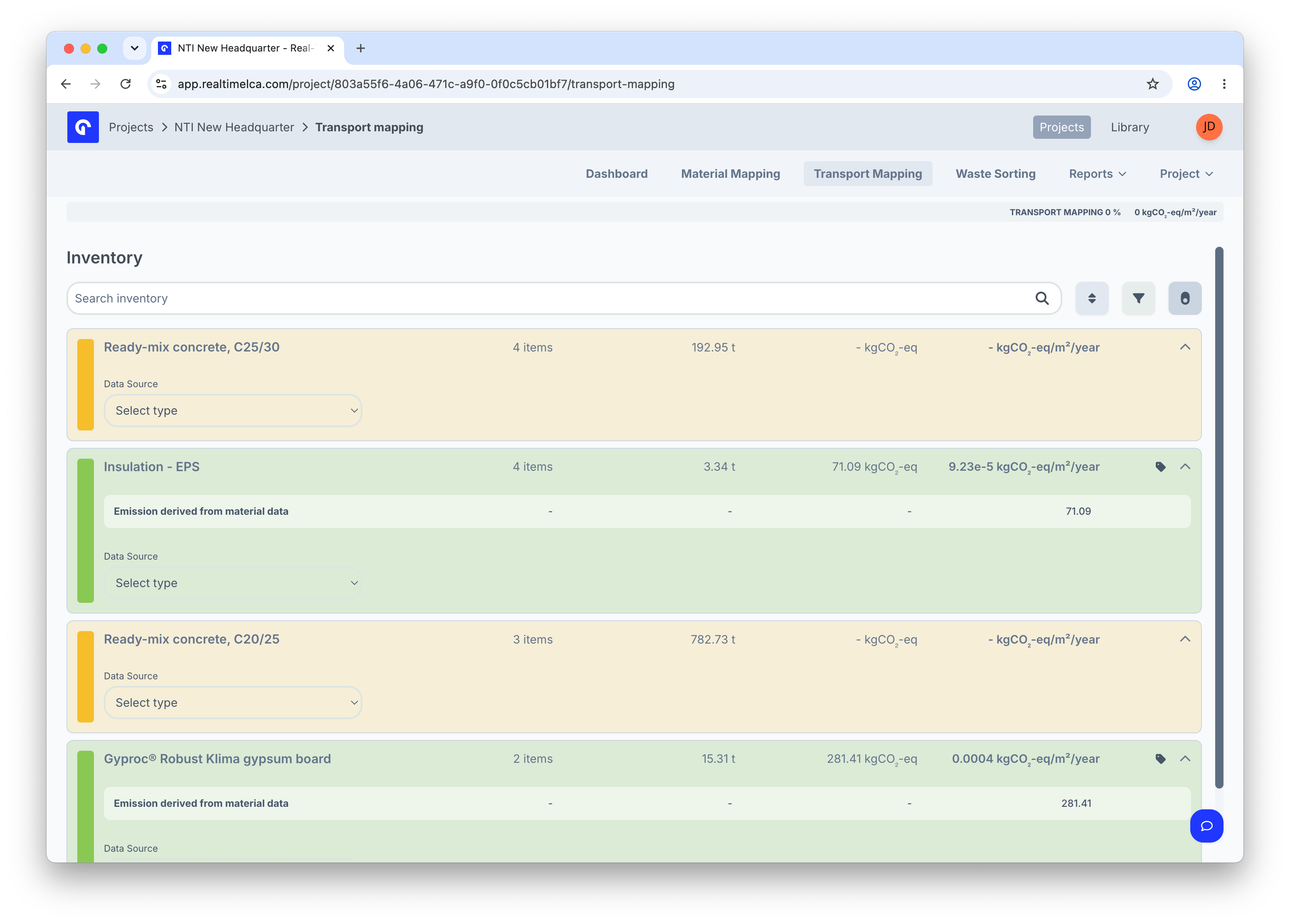
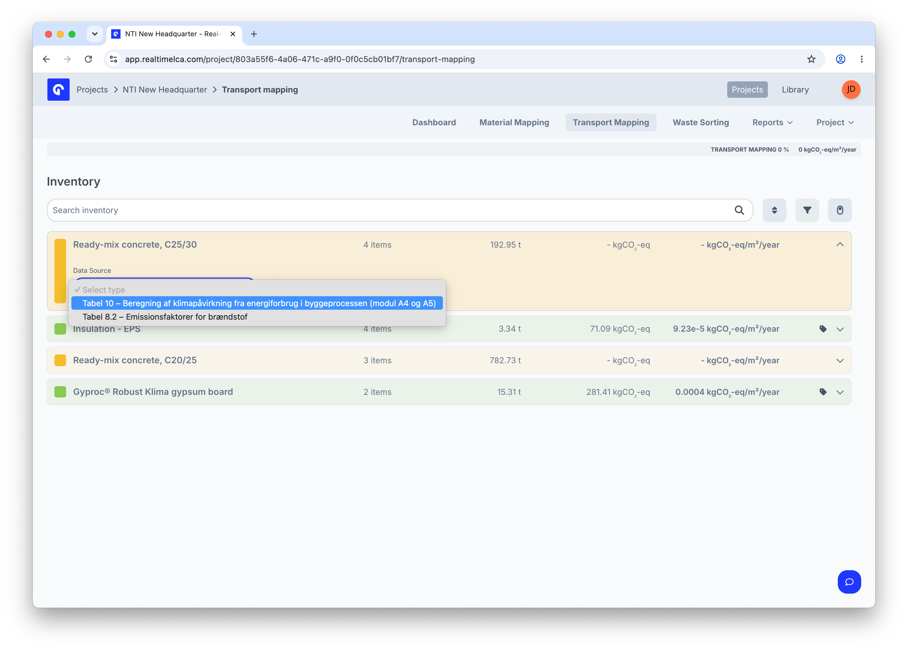
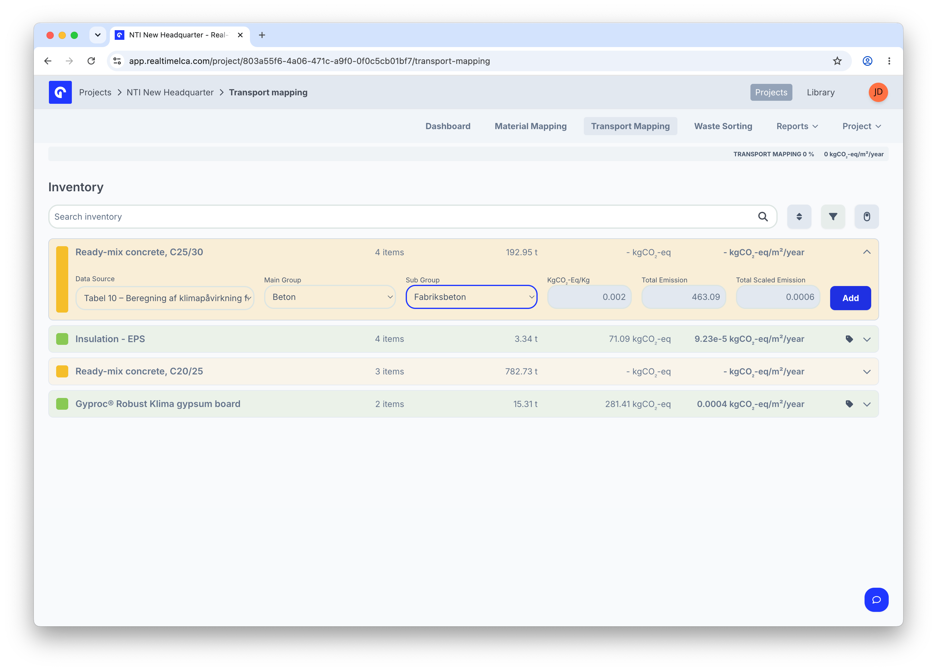
Map a transport type
Expand a row to open the assignment form. The flow is:- Pick a Data Source — the table the emission factor comes from (for example, a distance-based table or a fuel-based table).
- Pick a Main Group and Sub Group to narrow down to a specific transport type.
- Review the calculated kgCO₂-eq/Kg, Total Emission, and Total Scaled Emission columns.
- Click Add to commit.
Fuel-based emissions
Some regulations expose a fuel-based table — the emission is calculated from the volume or mass of fuel consumed per material instead of from a distance. Pick the fuel data source, choose an Emission Factor (for example, Diesel), and enter litres or kilograms.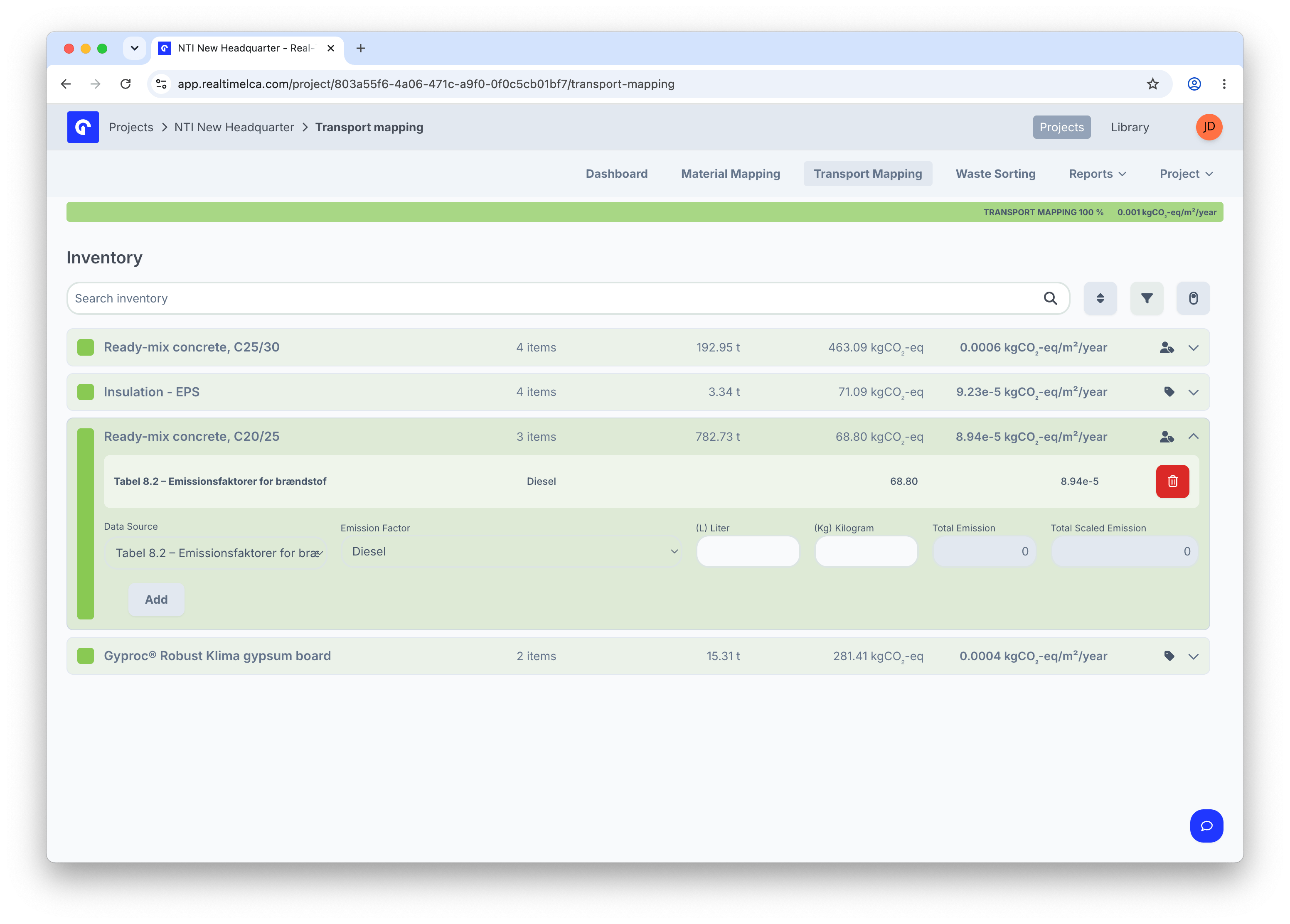
Material-derived data source
When a material’s EPD already includes module A4, Transport Mapping inherits the value automatically. The row shows an Emission derived from material data label and the Data Source picker is disabled — there is nothing to assign because the EPD already covers it.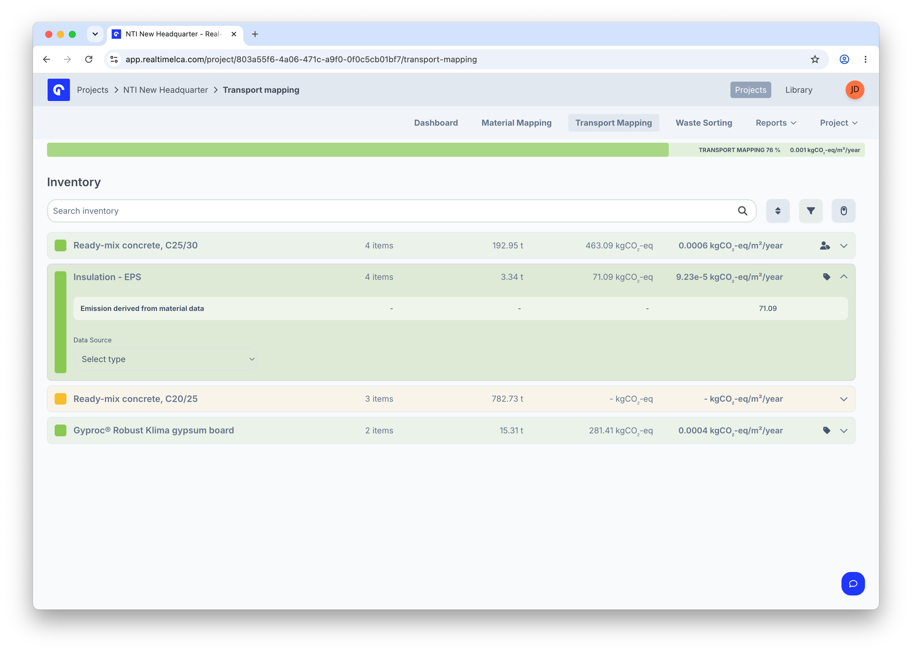
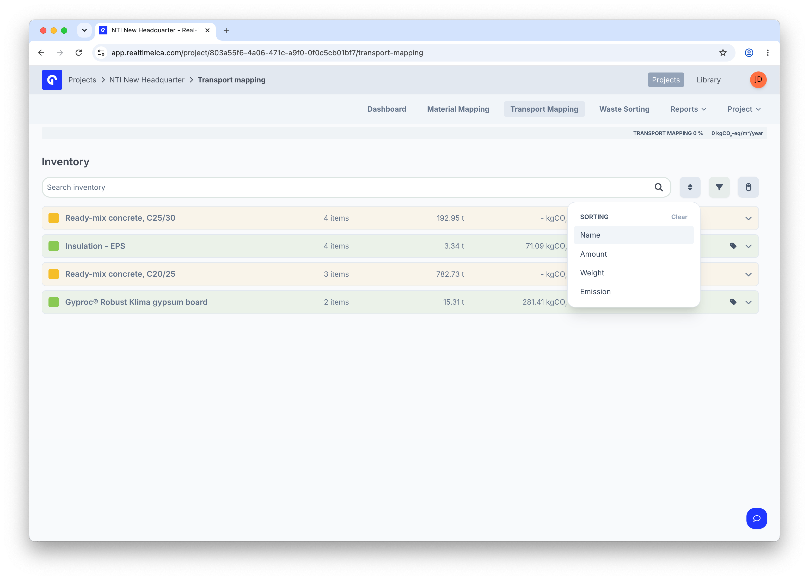
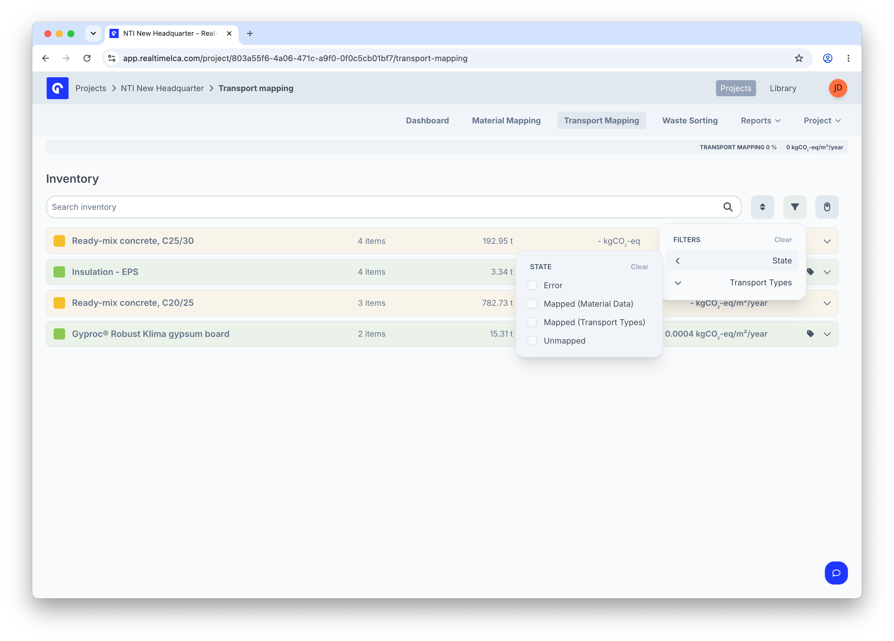
Search, sort, and filter
The toolbar above the inventory has the same shape as Material Mapping:- Search inventory — free-text search across material names.
- Sort — order the list by Name, Amount, Weight, or Emission.
- Filter — narrow by State (Error, Mapped (Material Data), Mapped (Transport Types), Unmapped) and Transport Types.